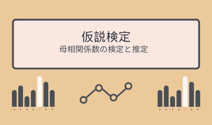
今回は2つの
相関関係の
関連度を
表す母相関係数の
検定と推定を
行う方法に
ついて説明致します
[PR]※本サイトには、プロモーションが含まれています
目次
相関関係とは?
1つの変数が変化すると
それに対応してもう1つの変数も変化する関係のことです
例えば
勉強を頑張った分だけ
テストの点数がよくなった
データがあります。
我々はそれを見て
勉強時間が変化すれば
テストの点数も変化すると考えます
つまり勉強時間とテストの点数は相関関係があると
いうことです
散布図(Scatter Plot)とは?
散布図(Scatter Plot)は
2つの連続的な変数(数値データ)の関係を
視覚的に表現するためのデータ可視化手法です。
横軸に1つの変数、縦軸にもう1つの変数を配置し
データポイントを点としてプロットすることで
変数間の相互関係やパターンを直感的に理解しやすくします。
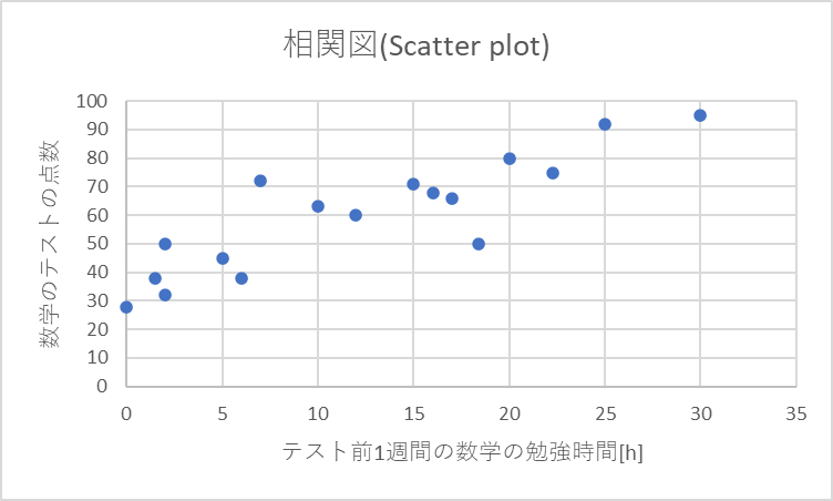
この散布図を見ると
テストを頑張った
人ほど点数が
良くなってる
ように見えるね!
相関係数(Correlation Coefficient)
xとyの関係を定量的に示すために
相関係数rを次のように計算する
\(\displaystyle r = \frac{S_{xy}}{S_{xx}S_{yy}}\)
\(S_{xx}\),\(S_{yy}\)は各変数の平方和
\(S_{xy}\)はxとyの偏差平方和
\(\displaystyle S_{xy}=\sum_{i=1}^{n}x_iy_i -\frac{\sum x_i\sum y_i}{n}\)
\(\displaystyle S_{xx}=\sum_{i=1}^{n}x_i^2 -\frac{(\sum x_i)^2}{n}\)
\(\displaystyle S_{yy}=\sum_{i=1}^{n}y_i^2 -\frac{(\sum y_i)^2}{n}\)
母相関係数に関する検定と推定
母相関係数
相関分析を行う2変数x,yは
\(N(μ_x,σ_x^2)\) , \(N(μ_y,σ_y^2)\)に従うと考え
xとyの母集団の相関関係を示す統計量として
\(\displaystyle ρ = \frac{C(x,y)}{\sqrt{V(x)V(y)}}\)
\(-1≦ ρ ≦ 1\)
Rの分布
Rは統計量で確率分布に従っている
\(ρ = 0\), 無相関の時
\(\displaystyle t = \frac{r\sqrt{n-2}}{\sqrt{1-r^2}} \)は自由度n-2のt分布に従う
\(ρ \neq 0\)の時
\(\displaystyle Z = \frac{1}{2}ln\frac{1+r}{1-r}\)は近似的に\(\displaystyle N(\frac{1}{2}ln\displaystyle \frac{1+ρ}{1-ρ},\frac{1}{n-3})に従う\)
相関が
あるときと
ない時で
統計量が
全然違う~
特に統計量Zは”z変換”と呼ぶ
\(\displaystyle t = \frac{r\sqrt{n-2}}{\sqrt{1-r^2}} \)
からrの式に変換すると
\(\displaystyle r(Φ,P) = \frac{t(Φ,P)}{\sqrt{Φ+(t(Φ,P))^2}}\)
確率分布表で上記の値を参照することが出来る
母相関係数\(ρ\)に関する検定手順
無相関であると仮説を立てる
\(H_0 : ρ =0\)
対立仮説を立てる
\(H_0 : ρ \neq 0\)
有意水準を立てる
\(α = 0.05 or 0.01 \)
棄却域を決める
\(R: ❘ r ❘ ≧ r(Φ , α)\)
データから相関係数を求める
\(\displaystyle r = \frac{S_{xy}}{S_{xx}S_{yy}}\)
\(Φ = n-2\)
rが棄却域にあれば棄却し相関があると判断する
早速例題を解いて
行きましょ~
Let’s start !
例題
以下のデータに相関があるか検定を利用して確認せよ
| No. | 1 | 2 | 3 | 4 | 5 | 6 | 7 | 8 | 9 | 10 | 11 | 12 |
| x | 8 | 20 | 16 | 21 | 23 | 15 | 12 | 13 | 9 | 18 | 21 | 22 |
| y | 25 | 51 | 32 | 44 | 60 | 45 | 20 | 34 | 30 | 35 | 24 | 52 |
まず散布図にしてみます
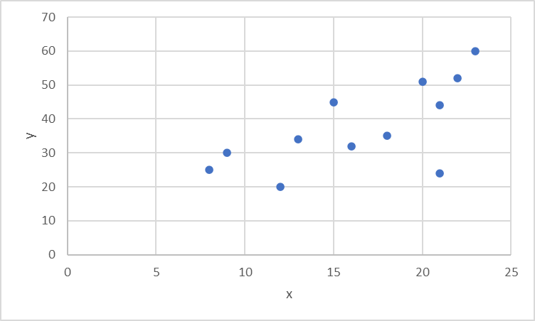
なんか
関係ありそう!!
仮説を立てる
相関がないと仮説を立てます。
\(H_0 : ρ = 0\)
対立仮説
\(H_1 : ρ \neq 0\)
有意水準と棄却域を立てる
有意水準
α = 0.05
棄却域
\(R: ❘ r ❘ ≧ r(10,0.05)\)
r分布表で上記の値を参照すると
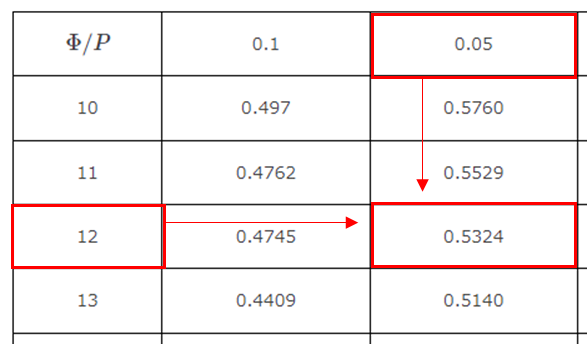
\(R: ❘ r ❘ ≧ 0.53\)
相関係数をデータから計算する
\(\displaystyle r = \frac{S_{xy}}{S_{xx}S_{yy}}\)
\(r =0.677\)
判定をする
\(R: ❘ r ❘ ≧ 0.53\)より
帰無仮説は棄却され
相関があると言える
でっきた~
次に母相関係数の
点推定と
区間推定を
やるよ~
母相関係数の推定手順
点推定は
\(\hat ρ = r\)
次に母相関係数の
区間推定を
やるよ~
Z変換
rをzに変換する
\(\displaystyle Z = \frac{1}{2}ln\frac{1+r}{1-r}\)
\(\displaystyle Z = \frac{1}{2}ln\frac{1+ρ}{1-ρ}\)の信頼区間を求める
(\(Z-\displaystyle \frac{1.96}{\sqrt{n-3}},Z+\displaystyle \frac{1.96}{\sqrt{n-3}})\) \(=(ζ_1,ζ_2)\)
信頼区間99%の時は1.96を2.576
90%の時は1.645
\(ρ\)の信頼区間を構成する
\(\displaystyle (\frac{e^2ζ_1-1}{e^2ζ_1+1},\frac{e^2ζ_2-1}{e^2ζ_2+1})\)
参考文献
第7章 相関分析