今回は
単回帰分析を
解析ソフトRを
利用して
単回帰モデルの
分析を行って
行きます
[PR]※本サイトには、プロモーションが含まれています
目次
解析に利用するR言語とは
R言語(R language)は
統計解析やデータ可視化など
で使用されるプログラミング言語の一つです
Rは、統計学者やデータ分析者など
データサイエンスや
統計解析の領域で広く利用されています。
Rを利用して単回帰直線の推定,描画をする
製品の特性値yと
焼成温度xの関係性を
解析用ソフトRを利用して
単回帰モデルの推定と
回帰直線を引いていきます
| サンプル番号 | x | y |
| 1 | 1030 | 9.1 |
| 2 | 1110 | 10.7 |
| 3 | 990 | 8 |
| 4 | 1000 | 8.2 |
| 5 | 1090 | 10.4 |
| 6 | 1030 | 10.5 |
| 7 | 1130 | 10.5 |
| 8 | 1080 | 9.9 |
| 9 | 1070 | 9.5 |
| 10 | 1110 | 10.3 |
データを成形する
データの入ったファイルを作っていきます
今回はdata1.csvというファイルに
データを格納していきます。
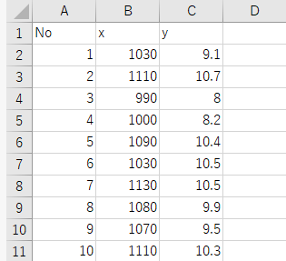
ファイルのアドレスはD:\data1.csv
データをRで読み込む
上記のファイルを読み込みます
# データを読みこむ
data <- read.csv("D:\\data1.csv")
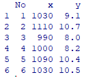
# 先頭の行を読み込む
head(data)headで先頭6行でデータが読み込まれているか確認します
単回帰モデルの実行と回帰係数を推定する
# データのラベルを直接呼び出すコマンド
attach(data)

# 単回帰モデルの実行
res = lm(y ~ x)


# 最小二乗法を利用した回帰係数の推定
res 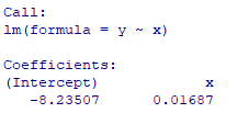
単回帰直線は
\(y=\hat β_1x+\hat β_0\)
上記の結果を見ると
\(\hat β_1=0.01687\)
\(\hat β_0=-8.23\)
# 散布図と回帰直線の作画
plot(x , y)
abline(res) 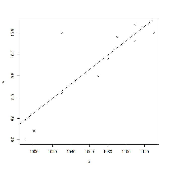
予測値の計算
# 予測値の計算x = 1120の時
predict(res,newdata = data.frame(x = 1120))
残差分析
# 標準化残差の取得
standardized_residuals <- rstandard(res)

# 標準化残差プロットの作成
plot(x, standardized_residuals, main = "標準化残差プロット", xlab = "説明変数", ylab = "標準化残差")

# ゼロラインを追加
abline(h = 0, col="red", lty = 2)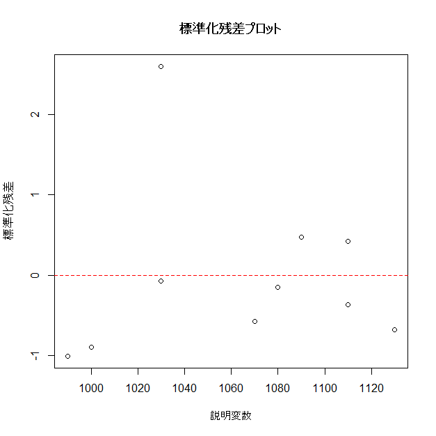
コードのまとめ
# データを読みこむ
data <- read.csv("D:\\data1.csv")
# 先頭の行を読み込む
head(data)
# データのラベルを直接呼び出すコマンド
attach(data)

# 単回帰モデルの実行
res=lm(y ~ x)

# 最小二乗法を利用した回帰係数の推定値
res

# 散布図と回帰直線の作画
plot(x, y)
abline(res)

# 予測値の計算 , x = 1120の時
predict(res,newdata = data.frame(x = 1120))

# 標準化残差の取得
standardized_residuals <- rstandard(res)

# 標準化残差プロットの作成
plot(x, standardized_residuals, main = "標準化残差プロット", xlab = "説明変数", ylab = "標準化残差")

# ゼロラインを追加
abline(h = 0, col = "red", lty = 2)
Summaryを用いて解析
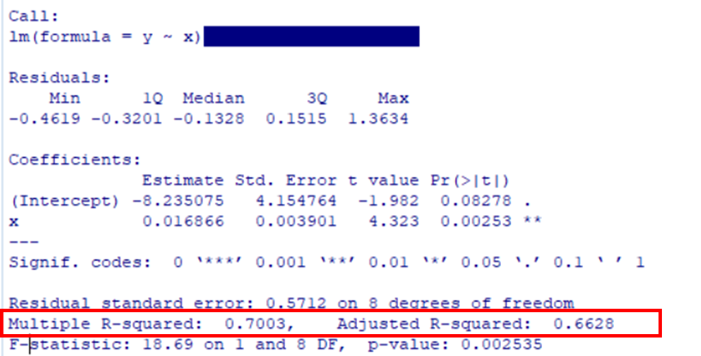
RではSummaryを用いることによって
回帰係数,決定係数の計算,
回帰係数の検定を行うことが出来る
# データを読みこむ
data <- read.csv("D:\\data1.csv")

# 先頭の行を読み込む
head(data)

# 単回帰モデルの実行
res=lm(y ~ x)


# 回帰分析
summary(res)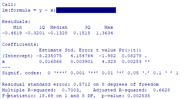
一つずつ
見ていきます
回帰係数を確認する
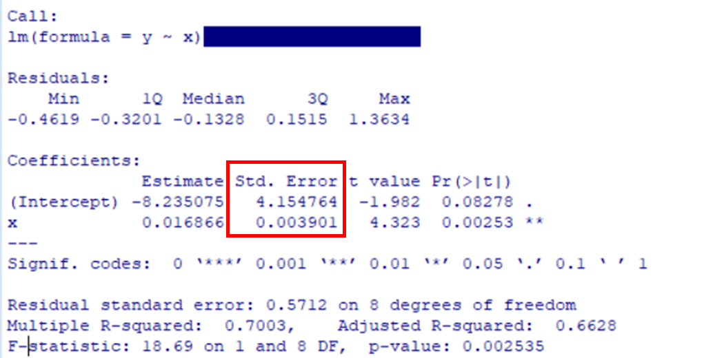
Estimateが回帰係数 \(\hat B_0=-8.23\), \(\hat B_1=0.016\)
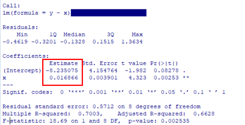
st.Errorは各回帰係数の標準誤差
回帰係数の検定を行う
t 値は帰無仮説\(H_0:β=0\)
としたときの検定統計量である
\(\displaystyle t=\frac{\hat β}{se(\hat β)}\)
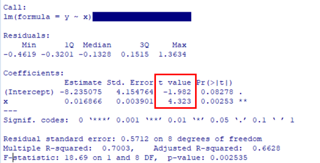
\(H_0:β_0=0\)と仮定したとき
\(\hat B_0=-8.23\)より極端な値になる確率は0.082
\(H_0:β_1=0\)と仮定したとき
\(\hat B_1=0.016\)より極端な値になる確率は0.00253
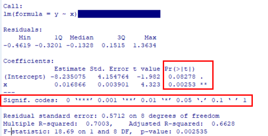
singif. codesは有意水準を示している
\(β_0\)は . なので有意水準0.1で有意である
\(β_1\)は ** なので有意水準0.01で有意である
この結果から
帰無仮説が棄却できるので2変数間の関係性はあると判断できる
決定係数
Multiple R-squaredは決定係数\(R^2=0.7\)
自由度調整済み決定係数\(R’^2=0.66\)
回帰係数の当てはまりはそこそこ良い