
今回は回帰直線の
残差と平方和に
ついて考えていきます
[PR]※本サイトには、プロモーションが含まれています
目次
回帰直線 の残差とは?
観測値\( y_i\) と
回帰直線によって
予測された値 \(\hat{y}_i\)
の差が残差です
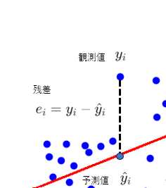
\(e_i = y_i – \hat y_i\)
総平方和(Total Sum of Squares)
観測値\(y_i\)が平均\(\hat y_i\)
からどれだけ離れているか
を示すもので
回帰分析ではyの平方和\(S_{yy}\)を総平方和と考える
\(\displaystyle S_T=S_{yy}=\sum_{i=1}^{n}( y_i-\bar y)^2\)
平方和の分解
総平方和は
回帰による変動成分と
残差による変動成分に
分解することが出来る
\(\displaystyle S_T=S_{yy}=\sum_{i=1}^{n}( y_i-\bar y)^2\)
\(=\displaystyle \sum(y_i-\hat B_0 – \hat B_1x_i)^2 +\sum(\hat B_0 + B_1x_i – \hat y)^2\)
\(=\displaystyle S_e(残差平方和)+S_R(回帰による平方和)\)
\(\displaystyle S_T = S_e(残差平方和)+S_R(回帰による平方和)\)
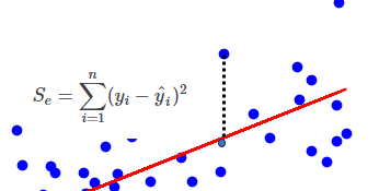
残差平方和(Residual Sum of Squares, RSS)
“観測値と回帰方程式によって予測される値との差の二乗
を合計したもの”
平方和は、回帰モデルが観測データをどれだけよく説明できているかを示す指標
\(\displaystyle S_e=\sum_{i=1}^{n} (y_i-\hat y_i)^2\)
観測値と予測値の差の
二乗なので値の
大きさで回帰モデルが
観測値をどれだけ
説明できているか
定量的に
判断できるようになったね
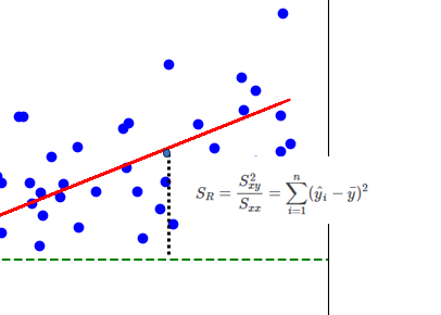
回帰平方和(Regression Sum of Squares, SSR)
“回帰方程式によって予測される値と観測値の平均値との差の二乗
を合計したもの”
回帰平方和は、回帰モデルによって説明される変動の大きさを示す
\(\displaystyle S_R=\frac{S_{xy}^2}{S_{xx}}=\sum_{i=1}^{n}(\hat y_i-\bar y)^2\)
直線と平均値の差の
二乗なので値の大きさで
回帰モデルの変動を
定量的に確認できるね
決定係数
回帰の寄与率は、通常
決定係数\(R^2\)(coefficient of determination)
によって評価されます。
決定係数は
“回帰モデルが観測データをどれくらいよく説明できるか”
を示す指標でありモデルの寄与度を定量化します。
\(\displaystyle R^2=1-\frac{S_e}{S_{T}}\)
残差\(S_e\)が小さいと
観測値と回帰方程式によって予測される値との差
が少ないということなので
“回帰直線がデータに当てはまっているほど”
\(R^2\)は1になり逆に当てはまっていないと
0に近くなりモデルの説明力が低いことを示します。
\(R^2\)が0.8であれば
80%の観測データの変動が回帰モデルによって説明されており
残りの20%は説明されていない(残差によるもの)
と解釈できる
参考文献

第7章 単回帰分析